Meta Learning in PyTorch

Nov 7, 2018

Got an image recognition problem? A pre-trained ResNet is probably a good starting point. Transfer learning, where the weights of a pre-trained network are fine tuned for the task at hand, is widely used because it can drastically reduce both the amount of data to be collected and the total time spent training the network. But ResNet wasn't trained with the intention of being a good starting point for transfer learning. It just so happens that it works well. But what if a network is trained specifically to obtain weights that are good for generalizing to a new task? That's what meta learning aims to do.

The usual setting in meta learning involves a distribution of tasks. During training, a large number of tasks, but with only a few labeled examples per task, are available. At "test time", a new, previously unseen, task is provided with a few examples. Using only these few examples, the network must learn to generalize to new examples of the same task. In meta learning, this is accomplished by running a few steps of gradient descent on the examples of the new task provided during test. So, the goal of the training process is to discover similarities between tasks and find network weights that serve as a good starting point for gradient descent at test time on a new task.

Model Agnostic Meta Learning (MAML)

MAML differentiates through the stochastic gradient descent (SGD) update steps and learns weights that are a good starting point for SGD at test time. i.e.., gradient descent-ception. This is what the training loop looks like:

- randomly initialize network weights W
for it in range(num_iterations):
    - Sample a task from the training set and get a few
      labeled examples for that task
    - Compute loss L using current weights W
    - Wn = W - inner_lr * dL/dW
    - Compute loss Ln using tuned weights Wn
    - Update W = W - outer_lr * dLn/dW

To compute the loss Ln, the tuned weights Wn are used. But, notice that gradients of the loss with respect to the original weights dLn/dW are needed. Computing this involves finding higher-order derivatives of the loss with respect to the original weights W.

At test time:

- Given trained weights W and a few examples of a new task
- Compute loss L using weights W
- Wn = W - inner_lr * dL/dW
- Use Wn to make predictions for that task

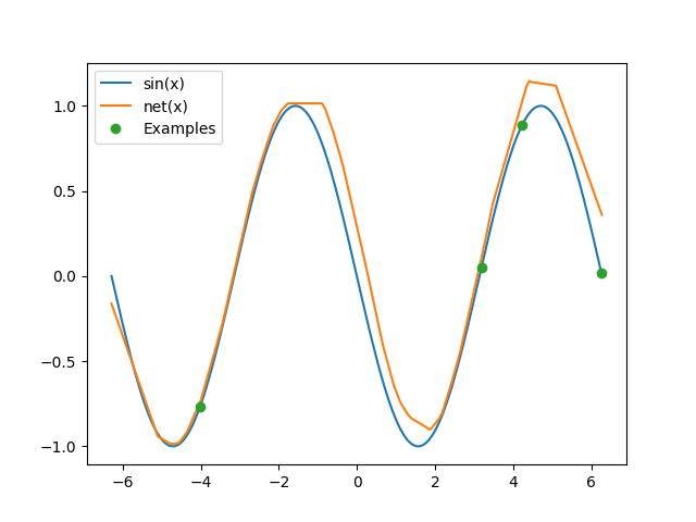
Let's try learning to generate a sine wave from only 4 data points. To keep it simple, let's fix the amplitude and frequency but randomly select the phase between 0 and 180 degrees. At test time, the model must figure out what the phase is and generate the sine wave from only 4 example data points.

import math
import random
import torch # v0.4.1
from torch import nn
from torch.nn import functional as F
import matplotlib as mpl
mpl.use('Agg')
import matplotlib.pyplot as plt

def net(x, params):
    x = F.linear(x, params[0], params[1])
    x = F.relu(x)

    x = F.linear(x, params[2], params[3])
    x = F.relu(x)

    x = F.linear(x, params[4], params[5])
    return x

params = [
    torch.Tensor(32, 1).uniform_(-1., 1.).requires_grad_(),
    torch.Tensor(32).zero_().requires_grad_(),

    torch.Tensor(32, 32).uniform_(-1./math.sqrt(32), 1./math.sqrt(32)).requires_grad_(),
    torch.Tensor(32).zero_().requires_grad_(),

    torch.Tensor(1, 32).uniform_(-1./math.sqrt(32), 1./math.sqrt(32)).requires_grad_(),
    torch.Tensor(1).zero_().requires_grad_(),
]

opt = torch.optim.SGD(params, lr=1e-2)
n_inner_loop = 5
alpha = 3e-2

for it in range(275000):
    b = 0 if random.choice([True, False]) else math.pi

    x = torch.rand(4, 1)*4*math.pi - 2*math.pi
    y = torch.sin(x + b)

    v_x = torch.rand(4, 1)*4*math.pi - 2*math.pi
    v_y = torch.sin(v_x + b)

    opt.zero_grad()

    new_params = params
    for k in range(n_inner_loop):
        f = net(x, new_params)
        loss = F.l1_loss(f, y)

        # create_graph=True because computing grads here is part of the forward pass.
        # We want to differentiate through the SGD update steps and get higher order
        # derivatives in the backward pass.
        grads = torch.autograd.grad(loss, new_params, create_graph=True)
        new_params = [(new_params[i] - alpha*grads[i]) for i in range(len(params))]

        if it % 100 == 0: print 'Iteration %d -- Inner loop %d -- Loss: %.4f' % (it, k, loss)

    v_f = net(v_x, new_params)
    loss2 = F.l1_loss(v_f, v_y)
    loss2.backward()

    opt.step()

    if it % 100 == 0: print 'Iteration %d -- Outer Loss: %.4f' % (it, loss2)

t_b = math.pi #0

t_x = torch.rand(4, 1)*4*math.pi - 2*math.pi
t_y = torch.sin(t_x + t_b)

opt.zero_grad()

t_params = params
for k in range(n_inner_loop):
    t_f = net(t_x, t_params)
    t_loss = F.l1_loss(t_f, t_y)

    grads = torch.autograd.grad(t_loss, t_params, create_graph=True)
    t_params = [(t_params[i] - alpha*grads[i]) for i in range(len(params))]


test_x = torch.arange(-2*math.pi, 2*math.pi, step=0.01).unsqueeze(1)
test_y = torch.sin(test_x + t_b)

test_f = net(test_x, t_params)

plt.plot(test_x.data.numpy(), test_y.data.numpy(), label='sin(x)')
plt.plot(test_x.data.numpy(), test_f.data.numpy(), label='net(x)')
plt.plot(t_x.data.numpy(), t_y.data.numpy(), 'o', label='Examples')
plt.legend()
plt.savefig('maml-sine.png')

Here is the sine wave the network constructs after looking at only 4 points at test time:

There's a variant of the MAML algorithm called FO-MAML (first-order MAML) that ignores higher-order derivatives. Reptile is a similar algorithm proposed by OpenAI that's simpler to implement. Check out their javascript demo.

Domain Adaptive Meta Learning (DAML)

DAML uses meta learning to tune the parameters of the network to accommodate large domain shifts in the input. This method also doesn't need labels in the source domain!

Consider a neural network that takes x as input and produces y = net(x). The source domain is a distribution from which the input x maybe drawn from. Likewise, the target domain is another distribution of inputs. Domain adaptation is what has to be done to get the network to work when the distribution of the input is changed from the source domain to the target domain. The idea in DAML is to use meta learning to tune the weights of the network based on examples in the source domain so that the network can do well on examples drawn from the target domain. During training, unlabeled examples from the source domain and the corresponding examples with labels in the target domain are available. This is the training loop of DAML:

- randomly initialize network weights W and the adaptation
  loss network weights W_adap
for it in range(num_iterations):
    - Sample a task from the training set
    - Compute adaptation loss (L_adap) using (W, W_adap) and 
      unlabeled training data in the source domain
    - Wn = W - inner_lr * dL_adap/dW
    - Compute training loss (Ln) from labeled training data
      in the target domain using the tuned weights Wn
    - (W, W_adap) = (W, W_adap) - outer_lr * dLn/d(W, W_adap)

Since we don't have labeled data in the source domain, we must also learn a loss function L_adap parameterized by W_adap.

At test time:

- Given trained weights (W, W_adap) and a few unlabeled
  examples of a new task
- Compute adaptation loss (L_adap) using weights (W, W_adap) and
  unlabeled examples in the source domain
- Wn = W - inner_lr * dL_adap/dW
- Use Wn to make predictions for that task for new inputs in
  the target domain

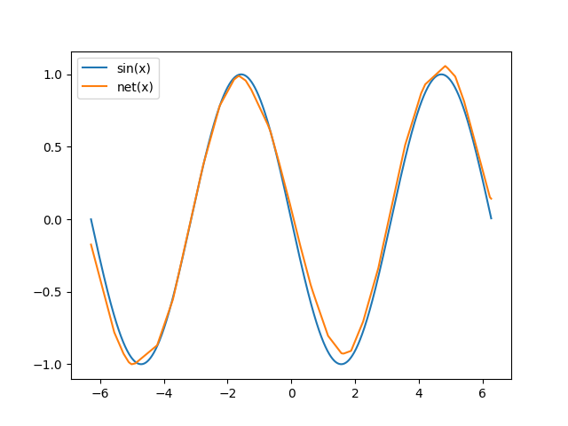
Once again, let's try learning to generate sine waves. In the target domain, the input, x, to the network is drawn from a uniform distribution [-2*PI, 2*PI], and the network has to predict y = sin(x) or y = sin(x + PI). Whether the network must predict y = sin(x) or y = sin(x + PI) has to be inferred from a single unlabeled input in the source domain. In the source domain, the input, x, to the network will be drawn uniformly from [PI/4, PI/2] to specify that zero phase is what we want and an input drawn from [-PI/2, -PI/4] shall specify that a 180 degree phase is desired. The source domain input is used to find gradients of weights with respect to the learnt adaptation loss, and a few steps of gradient descent tunes the weights of the network. Once we have the tuned weights, they can be used in the target domain to predict a sine wave of the desired phase.

import math
import random
import torch # v0.4.1
from torch import nn
from torch.nn import functional as F
import matplotlib as mpl
mpl.use('Agg')
import matplotlib.pyplot as plt

def net(x, params):
    x = F.linear(x, params[0], params[1])
    x1 = F.relu(x)

    x = F.linear(x1, params[2], params[3])
    x2 = F.relu(x)

    y = F.linear(x2, params[4], params[5])

    return y, x2, x1

def adap_net(y, x2, x1, params):
    x = torch.cat([y, x2, x1], dim=1)

    x = F.linear(x, params[0], params[1])
    x = F.relu(x)

    x = F.linear(x, params[2], params[3])
    x = F.relu(x)

    x = F.linear(x, params[4], params[5])

    return x

params = [
    torch.Tensor(32, 1).uniform_(-1., 1.).requires_grad_(),
    torch.Tensor(32).zero_().requires_grad_(),

    torch.Tensor(32, 32).uniform_(-1./math.sqrt(32), 1./math.sqrt(32)).requires_grad_(),
    torch.Tensor(32).zero_().requires_grad_(),

    torch.Tensor(1, 32).uniform_(-1./math.sqrt(32), 1./math.sqrt(32)).requires_grad_(),
    torch.Tensor(1).zero_().requires_grad_(),
]

adap_params = [
    torch.Tensor(32, 1+32+32).uniform_(-1./math.sqrt(65), 1./math.sqrt(65)).requires_grad_(),
    torch.Tensor(32).zero_().requires_grad_(),

    torch.Tensor(32, 32).uniform_(-1./math.sqrt(32), 1./math.sqrt(32)).requires_grad_(),
    torch.Tensor(32).zero_().requires_grad_(),

    torch.Tensor(1, 32).uniform_(-1./math.sqrt(32), 1./math.sqrt(32)).requires_grad_(),
    torch.Tensor(1).zero_().requires_grad_(),
]

opt = torch.optim.SGD(params + adap_params, lr=1e-2)
n_inner_loop = 5
alpha = 3e-2

for it in range(275000):
    b = 0 if random.choice([True, False]) else math.pi

    v_x = torch.rand(4, 1)*4*math.pi - 2*math.pi
    v_y = torch.sin(v_x + b)

    opt.zero_grad()

    new_params = params
    for k in range(n_inner_loop):
        f, f2, f1 = net(torch.FloatTensor([[random.uniform(math.pi/4, math.pi/2) if b == 0 else random.uniform(-math.pi/2, -math.pi/4)]]), new_params)
        h = adap_net(f, f2, f1, adap_params)
        adap_loss = F.l1_loss(h, torch.zeros(1, 1))

        # create_graph=True because computing grads here is part of the forward pass.
        # We want to differentiate through the SGD update steps and get higher order
        # derivatives in the backward pass.
        grads = torch.autograd.grad(adap_loss, new_params, create_graph=True)
        new_params = [(new_params[i] - alpha*grads[i]) for i in range(len(params))]

        if it % 100 == 0: print 'Iteration %d -- Inner loop %d -- Loss: %.4f' % (it, k, adap_loss)

    v_f, _, _ = net(v_x, new_params)
    loss = F.l1_loss(v_f, v_y)
    loss.backward()

    opt.step()

    if it % 100 == 0: print 'Iteration %d -- Outer Loss: %.4f' % (it, loss)

t_b = math.pi # 0

opt.zero_grad()

t_params = params
for k in range(n_inner_loop):
    t_f, t_f2, t_f1 = net(torch.FloatTensor([[random.uniform(math.pi/4, math.pi/2) if t_b == 0 else random.uniform(-math.pi/2, -math.pi/4)]]), t_params)
    t_h = adap_net(t_f, t_f2, t_f1, adap_params)
    t_adap_loss = F.l1_loss(t_h, torch.zeros(1, 1))

    grads = torch.autograd.grad(t_adap_loss, t_params, create_graph=True)
    t_params = [(t_params[i] - alpha*grads[i]) for i in range(len(params))]

test_x = torch.arange(-2*math.pi, 2*math.pi, step=0.01).unsqueeze(1)
test_y = torch.sin(test_x + t_b)

test_f, _, _ = net(test_x, t_params)

plt.plot(test_x.data.numpy(), test_y.data.numpy(), label='sin(x)')
plt.plot(test_x.data.numpy(), test_f.data.numpy(), label='net(x)')
plt.legend()
plt.savefig('daml-sine.png')

This is the sine wave contructed by the network after domain adaptation:

---

Archive · RSS · Mailing list